ELS: latency based load balancer, part 1

Load Balancing
Most Spotify clients connect to our back-end via accesspoint which forwards client requests to other servers. In the picture below, the accesspoint has a choice of sending each metadataproxy request to one of 4 metadataproxy machines on behalf of the end user.

The client should get a quick reply from our servers, so if one machine becomes too slow, it should be avoided. Furthermore, overloading one machine while the remaining 3 are idle leads to worse user experience. The problem of choosing the right machine is called load balancing.
Round-Robin
Round-robin is about as simple as a load balancing strategy can get. With 4 machines, distribute load as follows: 1, 2, 3, 4, 1, 2, 3, 4, 1, …
The problem with this strategy is that slow machines get the same amount of load as fast ones. In the following example, the first machine is 10 times slower than the remaining ones.
Join the Shortest Queue (JSQ)
Join the shortest queue (JSQ) sends a request to a machine with the lowest number of outstanding requests. These are requests that haven’t returned yet, meaning that they are on the way to a machine, being processed by the machine or on the way back.
This strategy performs better than round-robin in the previous case.
JSQ completed in about 80 seconds while round-robin took 245, more than 3 times longer than JSQ.
However, JSQ performs worse than round-robin when machines are failing fast because they are answering quickly with a failed reply and their job queue is short. Such machines get the most traffic, as can be seen in the following example, where one machine fails 90% of requests.
JSQ gets 11 incorrect replies out of 27, while round-robin only gets 6 incorrect replies in the same test case.
Circuit Breakers to the Rescue!
Problems of round-robin and JSQ can be alleviated with circuit breakers. A circuit breaker monitors latency and failure rate of different machines. It takes a machine out of rotation if latency or failure rate are too high. Machines are added back to rotation when metrics improve.
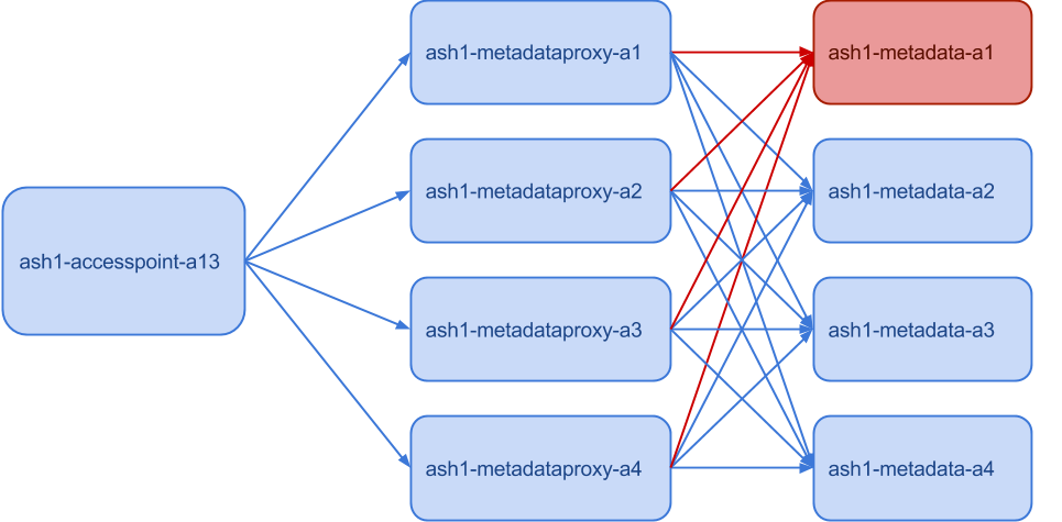
However, it’s easy to shoot yourself in the foot when the circuit breaker isn’t set up the right way. Suppose a circuit breaker activates when success rate is below 80% and we are in the situation that is showed on the picture below.Since one of the metadata machines is down (marked with red), the metadataproxy machines all get only 75% success rate. If we set the success rate threshold for the circuit breaker to 80%, we’ll shut down the whole metadataproxy service, even though it can still handle 75% of its maximum capacity.
Another hard thing about circuit breakers is that one needs to have sufficient confidence in the measured metrics. If you base your decision on the last 10 requests and it just happened that the last 3 requests failed, you’d trigger the circuit breaker with threshold of 80%, even though the previous 1000 requests were all okay. Having enough statistical confidence is harder than it seems at first.
Rainbows

Let’s talk about rainbows for a while. How many colors do you see in a rainbow?People typically answer between 5 and 7 depending on where they grew up, but the right answer is an infinite number1. It’s simpler to think of a small number of colors than an infinite number, so our brains slice the space of colors into a few discrete categories.
I believe that the same phenomenon is behind circuit breakers. Our lazy brains reduce infinity into a yes/no dichotomy. Like the rainbow, there are more colors to be seen. Just because our brains work this way doesn’t mean we have to write software the same way.
Expected Latency Selector (ELS)
Enter Expected Latency Selector, also known as ELS. It’s a probabilistic load balancer that we built for use in our backend services, where each machine has a weight. A machine with a 2 times higher weight gets twice as much traffic. Since each weight is a positive real number, we use an infinite space instead of a yes/no dichotomy. While it shares no code, it is in many ways similar to C3 for Cassandra.
ELS measures the following things.
- Success latency and success rate of each machine.
- Number of outstanding requests between the load balancer and each machine. These are the requests that have been sent out but we haven’t yet received a reply.
- Fast failures are better than slow failures, so we also measure failure latency for each machine.
Since users care a lot about latency, we prefer machines that are expected to answer quicker. ELS therefore converts all the measured metrics into expected latency from the client’s perspective. For simplicity, we are not going to show and explain the formula now, but we’ll do that in the second part of this blog post.
In short, the formula ensures that slower machines get less traffic and failing machines get much less traffic. Slower and failing machines still get some traffic, because we need to be able to detect when they come back up again.
As we shall see, it doesn’t have the problems outlined above for round-robin, JSQ and circuit breakers.
Benchmarks
Let’s look at benchmarks comparing round-robin, ELS and JSQ. We used three routers and 12 machines running a simple CPU-bound service with log-normal distribution of job sizes. Each router ran a different load balancer (round-robin, ELS and JSQ) and had its own designated 4 machines, so that the results were independent.
FIRST BENCHMARK
The first benchmark ran for 11 hours and started at no traffic and ended at 1100 requests per second (rps), which is slightly above the maximum throughput of the system, 1030 rps. Towards the end, the number of correct requests stopped growing while the number of failures increased.

Instead of simply looking at the average latency we look at the 75th and 99th percentile when evaluating benchmarks. For example, if the 99th percentile of latency is 47 milliseconds, 99% of requests get a reply in 47 milliseconds. These are more important metrics than average, since average latency can easily hide problems. You can have average latency 100 milliseconds even though 1% of requests take 5 seconds.
The 75th percentile of latency shows that there is little difference between ELS, JSQ and round-robin until the point when we reached about 50% of the capacity, when round-robin started being 30% slower than ELS and JSQ. At 75% of capacity, the difference became 100% and then occasionally rised up to 250%. On the other hand, there was very little difference between ELS and JSQ.

With the 99th percentile of latency, we notice round-robin being 50% slower already at 30% of capacity and then the slowness stayed at about 40-60% until about 90% capacity, when all load balancers lose breath. When the system is overloaded beyond its capacity, there is very little the load balancer can do. Every system ultimately saturates.
![99%-ile of latency]](https://storage.googleapis.com/production-eng/1/2015/11/10hour-latency-p99.png)
Even though all machines were supposed to be identical, in reality they weren’t. The reason remains unclear, but the most likely culprit is virtualization.
To get a more objective comparison of ELS and JSQ, we swapped the two machines running these load balancers. The graph below shows the 99th percentile of latency with the same setup, however notice that JSQ and ELS switched colors due to hardware swap.
JSQ was faster than ELS by about 20-30% when the load was between 50 and 90% of capacity. Otherwise they were comparable.

For the record, there was barely a difference in the 75th percentile of latency after the hardware swap.

SECOND BENCHMARK
For the second benchmark we kept the same setup as in the first benchmark, but we made three out of the 12 machines randomly fail 50% of all requests, so that each load balancer had one such failing machine. We also made the test shorter to only 5 hours.
With very low load, ELS had very low error rate, but it kept increasing steadily, while round-robin kept its error rate at about 12.5%. Note that with three machines, round-robin sends 1/4th of traffic to each machine. One of them fails one half of its requests, so we get failure rate of about 1/8 = 12.5% as expected.
The error rate of JSQ started at about 12.5% but then kept rising up to about 17.5%. This stems from the strategy that JSQ employs, as shown in the animation above.

When we look at the 75th percentile of latency, round-robin started losing breath at about 75% of the capacity while the latency of ELS and JSQ was very stable until the very end. JSQ has the best latency but it comes at the cost of the highest error rate of all three algorithms.

Note that the increasing error rate of ELS is a feature and not a bug! When the system is becoming more saturated and less responsive, it makes sense to send traffic to a machine that fails fast, because the Spotify client will do a retry.

One interesting thing about the previous graph is that the latency of round-robin is much more shaky than the latency of ELS and JSQ. This was also true in the first benchmark, but it’s not so apparent when using 10-minute resolution. Let’s look at the 75-th percentile in the first benchmark again, but this time with 1-minute resolution.
ELS and JSQ also have spikes, but they are much smaller and mostly happen when there is a spike in round-robin too. All benchmarks were run from the same machine that generated the load, so we suspect that there are network hiccups behind those spikes or jobs running in the background.
Relative circuit breaker
ELS also has an improved circuit breaker that doesn’t have the problem that we explained in the beginning. The circuit breaker takes a machine out of rotation if it performs badly relatively to the global average. In the example in the beginning, we had four machines all failing 25% of traffic, so each of them is equally good (bad) and the relative circuit breaker would’t trigger in that case. A machine would have to perform substantially worse than the global average of 75% to be excluded.
Pros and cons of ELS
LIMITATIONS
- Uses only locally observable information on the load balancer machine.
- 99th percentile of latency is more important for user experience, perhaps we should use that for calculating weight instead of expected (average) latency.
- Adding a slow machine to rotation can degrade performance, because it will always get some traffic.
- Not invented here syndrome? Perhaps, but C3: Cutting Tail Latency in Cloud Data Stores via Adaptive Replica Selection uses almost the same approach for Cassandra.
ADVANTAGES
- Great performance, almost as good as JSQ in benchmarks with non-failing machines. Outperforms JSQ when machines fail.
- Even though the weight formula uses expected (average) latency, we see good results for the 75th and 99th percentiles too.
- Uses only locally observable information (note that this item also appears in the list of limitations). This makes the code simpler and less error-prone.
- Has a relative circuit breaker that only triggers when a machine is worse relatively to the global average.
- Since we only use locally observable information, we don’t need to modify the 100+ Spotify backend services to get the load balancer to work.
- The technology has proved as very reliable in the half year we have used it.
To be continued
In part 2, we’ll go through more technical details like the weight formula that is the heart of the load balancer.
Footnotes
1. You could object that only finitely many photons reach your eye in a given time span, but the number is so big that we can assume that a rainbow has an infinite number of colors.
Tags: algorithm, backend, backend services, latency


